one matrix, many questions.
One linear recommender, a short formula, and the modeling choices hiding inside it.
archive date · Archive date selected by the author from the original notes; this version was prepared in October 2026. · text updated 2026-10-14
Give a model a user’s listening history and ask it to reconstruct that history. A wonderfully unhelpful answer is available: copy the input. Perfect reconstruction, no new music.
EASE blocks that answer with one constraint: an item cannot reconstruct itself. Its score has to come from other items in the history.
Its item-to-item matrix, B, turns a user’s history into recommendation scores:
scores = history @ BEach column of B contains the weights for one target item. The questions are how to learn those weights, what they mean, and what happens when the matrix gets too large to hold comfortably.
Block the easy answer
Take a user–item interaction matrix X. A row records a user’s history. A zero usually means that we did not observe an interaction; it does not automatically mean a dislike.
Harald Steck’s EASE learns a regularized linear reconstruction:
minimize ||X - X @ B||²_F + lambda * ||B||²_F
subject to diag(B) = 0
Without the constraint, the identity matrix would copy X exactly, although regularization would penalize its weights. Setting the diagonal to zero blocks that direct route. To reconstruct the column for one item, the model must use the other items. lambda controls how strongly large coefficients are penalized.
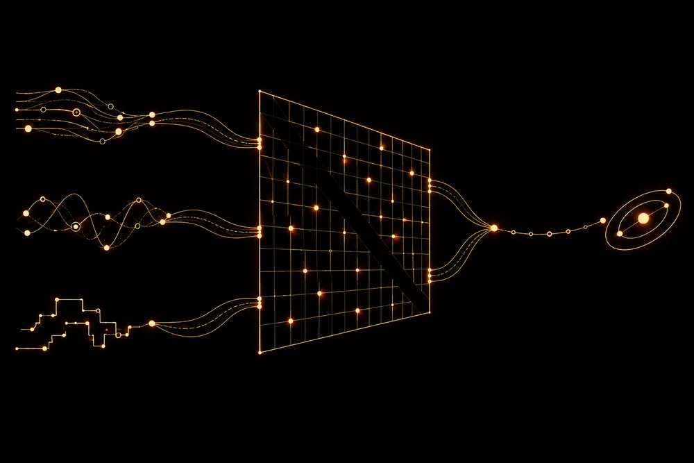
Where do the weights come from?
For positive lambda, define the regularized inverse:
P = inverse(X.T @ X + lambda * I)
B[i, j] = -P[i, j] / P[j, j]   # i != j
B[j, j] = 0
Steck’s closed-form solution puts the fit into an inverse and a column normalization. For target j, take column j of P, divide its off-diagonal entries by -P[j, j], and set the diagonal entry to zero. That gives the weights used to predict that target from the other items, without a training loop.
Even though P is symmetric, dividing its columns by different diagonal values can make B asymmetric. The weight from A to C need not equal the weight from C to A.
Each target is predicted from the other columns jointly. A coefficient is learned alongside those other predictors, so it is not just a count of how often two items appeared together.
What does one score mean?
For a target item, prediction is a sum of contributions from the history. In this example, the user has observed A and B, each with a history value of 1. With illustrative weights of 0.6 and 0.4, their contributions to unseen C add up to 1.0:
A negative coefficient would pull C’s score down. These values are useful for ordering candidates; a coefficient of 0.6 does not mean a 60% chance. The arrow from A to C shows a contribution to a score, not that A causes someone to like C.
The diagonal becomes a research question
The constraint has done its job: C cannot use its own history entry to reconstruct itself. But forcing every diagonal entry to exactly zero also raises a question about recommendation quality across the catalogue.
Moon and colleagues’ RLAE/RDLAE work replaces the equality with an upper bound: diag(B) <= xi. Their experiments connect that relaxation to recommendation quality for unpopular items. Whether it helps on a new dataset still needs measuring.
That suggests an experiment with a specific comparison: measure the effect separately on head and tail items. An aggregate metric can hide which part of the catalogue changed.
Which history goes into the matrix?
The weights are only half of history @ B. A binary interaction, a count, and a time-decayed history encode different things, even if they enter the same multiplication. With a binary history, observing A once or repeatedly supplies the same value. With counts, A’s contribution is scaled by the number of interactions. Whether that repetition is useful evidence or lets a few very active users dominate the statistics depends on the task.
This choice matters during fitting, where X determines the learned relationships, and during scoring, where the supplied history determines their contribution to each target. In our Avito solution, several versions of user history reused one learned matrix. The relationships stayed fixed while the evidence supplied at scoring time changed; each view did not need a separate fit.
The matrix also has a storage bill
A dense item-to-item matrix has quadratic storage in the catalogue size. For 100,000 items, one float32 matrix alone takes 100,000² × 4 bytes: 40 GB in decimal units, before the other matrices and workspace needed during fitting. This is a storage calculation, not a measured memory peak. Double the catalogue and that one matrix becomes four times larger.
My SANSA optimization notes pick up this computational side: which sparse products can be reused, which temporary allocations can disappear, and whether the resulting weights still match.