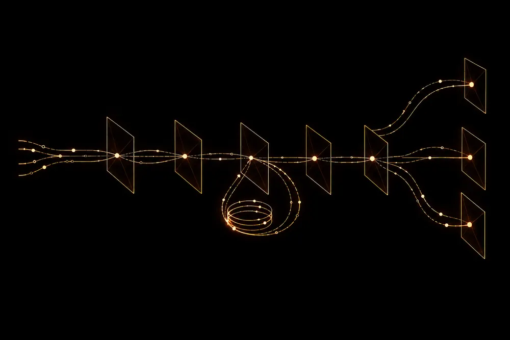
five models, one prediction loop.

Five models made the final prediction. Before any of them could run, the notebook had to answer a less glamorous question: what do we actually know about this learner right now?

In Riiid, each incoming batch carried new questions and revealed answers to the previous batch. A prediction depended on a learner’s changing history. We had to keep that history moving without letting an answer that had not arrived yet sneak into its features.

Our team finished 37th in Kaggle’s Riiid Answer Correctness Prediction competition. My published 2gbm_3nn notebook, with Dean listed as an editor, contains the assembled inference loop. The transformer experiments have their own teammate write-up.

Answers arrive one batch later

The main loop keeps copies of the previous batch for the tree and neural branches. On the next iteration, it attaches the newly revealed correctness labels and chosen responses. Only then can it update answer-dependent statistics.

This is the order, in shortened pseudocode:

for batch in test_stream:
    if previous exists:
        previous.answers = batch.prior_group_answers_correct
        update_answer_statistics(previous.questions)
    features = read_history_and_observed_events(batch)
    submit_predictions(batch.questions, features)
    previous = batch

Counts of correct answers, recent accuracy, and timestamps of correct or incorrect responses follow that delayed update. Observable events, such as encountering a question or lecture, can update separate counters immediately. Keeping those two kinds of state apart matters: a timestamp is available when a question arrives, while its correctness label is still hidden.

The code also keeps separate preprocessing copies. Missing elapsed time becomes zero for SAINT, while the tree branch uses a stored mean of about 25.5 seconds. Each branch receives the representation expected by its pipeline.

Several memories of the same learner

The tree features describe history at different resolutions. There is overall user accuracy, accuracy on the last 5, 20, and 50 questions, and separate session histories that reset after gaps of 3, 12, or 48 hours. A difficult recent stretch can therefore coexist with a strong long-term record in the feature vector.

Question and subject statistics add another reference point. The pipeline tracks repeated attempts, subject-part accuracy, lecture exposure, and time since the last correct or incorrect answer. It also compares a user’s accuracy with a question’s historical accuracy, including a ratio and a harmonic mean.

For subject parts with fewer than ten observations, the update function smooths accuracy toward a default for that part. Its calculation simplifies to this pseudocode:

accuracy = (correct + (10 - count) * part_prior) / 10
# only while count < 10

One correct answer gets some credit without immediately becoming a perfect estimate of subject mastery. These features enter the ensemble together; the notebook does not contain a feature-by-feature ablation.

History has a storage bill

Repeated user–question pairs use a SQLite table mapping the pair to an index. A separate array stores the last timestamp at that index. A returning pair retrieves its timestamp, produces a time difference, and updates the array. A new pair gets an index and a database row.

That separates the lookup from timestamp storage. It also means a SQL lookup per row, with a commit at the end of the feature pass. There is a practical cost to carrying fine-grained history through every batch.

The neural history has a more explicit compromise:

if (prev_test_df is not None) & (psutil.virtual_memory().percent < 90):
    # update stored sequences from the previous batch

This checks system RAM usage. At 90% or higher, the branch skips that history update. The stored sequence can become stale, but it avoids additional work under memory pressure. We cannot put a score gain on this guard from the notebook alone.

Three clocks and a spare zero

SAINT’s encoder combines question, subject-part, position, and explanation embeddings. Its decoder combines position, previous response, elapsed time, and three lag embeddings. The lag representations use seconds capped at 300, minutes capped at 1,440, and days capped at 365.

The teammate’s write-up discusses categorical time embeddings and separating padding from real zeros. The notebook shifts question IDs, historical responses, and explanation flags by one. After packing history into padded buffers, TestDataset aligns its inputs like this:

exercise = np.append(q[2:], [target_id+1])
response = res[1:]

The target question gets preceding response history. With 100-slot buffers, these inputs have 99 positions. An upper-triangular mask blocks attention to future positions in encoder, decoder, and cross-attention.

These details let the model receive several scales of time while preserving the sequence’s prediction order. Stored histories are capped at 100 events.

Five models share the final answer

The notebook loads LightGBM, CatBoost, and three SAINT checkpoints. Two SAINT instances have two encoder and decoder layers each; the third has three. All use 256-dimensional embeddings. Inference takes the last position’s sigmoid probability from each neural model.

The actual blend is:

p = 0.175 * lightgbm + 0.075 * catboost
  + 0.25 * (saint1 + saint2 + saint3)

The teammate reports public scores of 0.794, 0.799, and 0.804 for LightGBM, a transformer, and blending respectively. The notebook page separately displays a rounded private score of 0.806.

The ensemble equation fits on two lines. Making those five probabilities arrive at the right moment takes considerably more bookkeeping: answers one batch late, several versions of history, and a memory budget that gets a vote too.